If you store GPS coordinates as 32-bit floats, your precision in Iowa is about two feet. In central London the precision drops to half a millimeter, and at the South Pole it’s about a trillion times finer than the Planck Length.

Floating point types are the standard convention for representing continuous quantities in computing. There are other solutions like fixed point or symbolic representations, but floats are an all-purpose out-of-the-box solution for most applications. While they are flexible at multiple scales, that flexibility can lead to some interesting consequences, one of which this post will explain.

The application I want to discuss here is that of representing a point on the surface of the Earth as a (latitude, longitude) pair. When using floats to represent the lat/lon, the abstract numerical variation of floats is converted into a concretely measurable physical variation in distances.¹ I’ll start with some preliminaries:

Preliminary: Floating Point Types

For the rest of the post, I’ll use “float” to mean standard 32-bit floating points, though a similar analysis would make sense for other float types. The layout of a 32-bit float looks like this:

Source

The Wikipedia article goes into more detail (and is more technically correct), but basically it’s base-2 scientific notation: the exponent specifies a power of 2, and the mantissa is a number between 1 and 2, represented as bits after the binary point. In other words, the red part represents the “significant digits” of the number, while the green part represents the scale. This is what allows floats to be flexible at different scales, but also means that the absolute numerical precision of a number depends on the value of the number.

Getting a bit more concrete, the Unit of Least Precision (or ULP) is the size of the gap between two consecutive floating point numbers. For 32-bit floating points, the “fraction” (aka significand aka mantissa) consists of 23 bits. Thus, for a 32-bit float in the range $[2^n, 2^{n+1})$, the ULP is always exactly $2^{n-23}$.

So for example, if we take $x \sim$1 trillion, then $x \in [2^{39}, 2^{40})$; thus, the ULP is $2^{16}$. That is, consecutive floats in a neighborhood of $x$ are separated by gaps of size $2^{16} = 65,536$. As a matter of fact, the exact value of 1 trillion is not even representable as a float32; the two consecutive floats on either side of it are the integers 999,999,995,904 and 1,000,000,061,440.

More generally, the precision of any 32-bit float $x$ is always somewhere between $2^{-23}x$ and $2^{-24}x$, or $\frac{x}{8,388,608}$ and $\frac{x}{16,777,216}$. So, while the absolute precision is locally constant with discrete jumps at powers of 2, zooming out it roughly tracks something like $\frac{x}{12,000,000}$.

Preliminary: Geographic Coordinate Systems

In the standard convention used by most GPS providers (such as the one your phone uses), a physical position on the surface of the Earth is described by a pair of real numbers: latitude and longitude. Latitude ranges from $-90°$ to $+90°$, along meridians which span the south pole to the north pole. Longitude ranges from $-180°$ to $+180°$, with the two extremes meeting at the antimeridian.

As a consequence, while a degree latitude always represents the same physical distance

1° Latitude ~ 111km,

the physical distance of a degree longitude actually depends on which parallel you’re on, i.e. at what fixed latitude the parallel runs along. Along the equator, there is a similar conversion of 1° Longitude ~ 111km, but near the poles the parallels shrink down to nothing. So, the conversion between degrees Longitude and physical distance has an additional dependency on the current latitude. Fortunately, it has a fairly simple closed form:

1° Longitude ~ 111km * cos(Current Latitude),

where cos means the usual cosine.

Putting It Together: Physical Precision

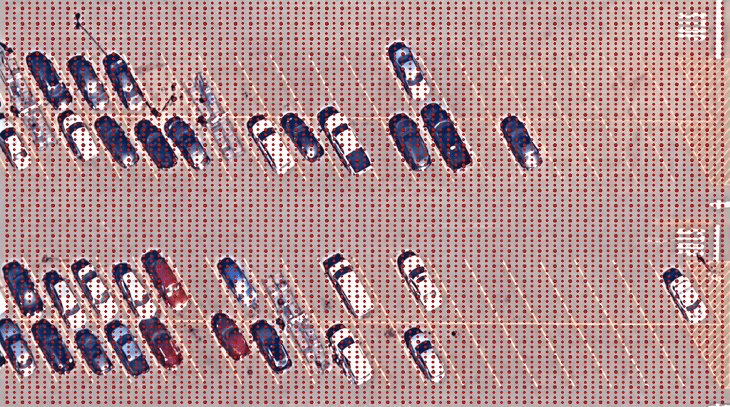
Putting the above together tells us that the physical precision of a floating point (lat, lon) pair depends on where in the world you are! So for example, here is a satellite image of a parking lot in my home state of Iowa, overlaid with a grid of dots representing the representable float32 lat/lons.²

On the other hand, here is a satellite image of the parking lot at the Palace of Westminster in London, overlaid with a grid of dots representing the representable float32 lat/lons:

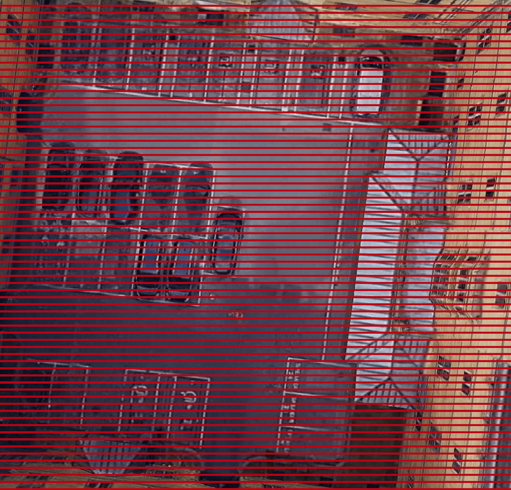
Well, these look more like stripes than a grid. The vertical spacing is actually about the same as in Iowa. The horizontal spacing between points was around 60cm (or 24in) in Iowa due to being contained in the longitudinal range $-[64, 128)° = -[2^6, 2^7)°$. On the other hand, the horizontal spacing at Westminster is about 0.5mm, or roughly 1000x finer, due to its position in the longitudinal range $-[0.0625, 0.125)° = -[2^{-4}, 2^{-3})°$. That’s because longitude gets extremely precise near the prime meridian (and similarly, latitude gets increasingly precise near the equator).

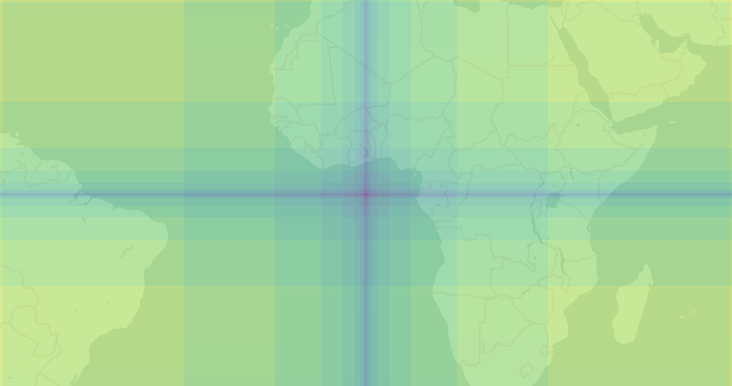
To illustrate this more globally, define the combined physical area precision at a given (lat, lon) to be the product of the respective physical precisions of the lat and lon separately. To put it another way, given a float32 lat/lon pair $(x,y)$, it is the area bounded by the rectangle with vertices

$(x,y), (x+ULP(x), y), (x+ULP(x), y+ULP(y)), (x, y+ULP(y)).$

Now, consider the following log-scale heatmap of the combined physical area precision, overlaid on a Mercator projection of the Earth (the image is a link to an interactive map):

A few things to note:

1. As one approaches the equator resp. prime meridian, the absolute precision of latitude resp. longitude in the floating point representation gets increasingly finer, creating the overall cross pattern.
2. At low zoom levels, one can further see a “plaid” grid pattern even away from the prime meridian/equator. This corresponds to the discrete jumps in absolute precision at powers of 2. That is, the jumps occur at $\pm 128$ degrees Longitude, and $\pm 64, 32, …, 1, 0.5, 0.25, 0.125, …$ degrees Latitude/Longitude.
3. Within a grid cell, one can actually see a subtle gradient, tending slightly greener as one moves towards the poles before the discrete jump back to yellow. This is due to the effect of latitude on the precision of longitude.
   • Thus, there are two counter-balancing forces in effect: a gradual increase in the physical precision of longitude as the parallels shrink, combined with decreases in the physical precision as latitude grows and crosses power-of-2 thresholds.

Finally, due to the limitations of the raster heatmap, there are two areas of the map which are worth describing in a bit more detail:

Null Island and the Planck Length

While the above heatmap gets pretty dark, it understates just how precise values get once the latitude and longitude actually reach 0. This happens for both coordinates at the lat/lon (0.0, 0.0), aka Null Island. Here, the float32 values dip into subnormal territory, where the ULP hits its minimum of $2^{-149}$. In physical terms, this translates to a precision of $10^{-40}$ meters. As a point of comparison, angstroms, which are used to measure sizes and distances between atoms, are a relatively coarse $10^{-10}$ meters. Even the Planck Length, the scale at which all known laws of physics are expected to break down, is roughly $10^{-35}$ meters. So the physical precision of float32 at Null Island is 100,000x more precise than that!

The Poles

In the default Mercator projection of the basemap, there is a cutoff around $\pm 85$ degrees latitude. This is for good reason, as the Mercator projection increasingly skews from physical reality as one approaches the poles. Unfortunately, that also cuts off some additional interesting behavior. I’ve created a visual to better illustrate what happens at the poles.

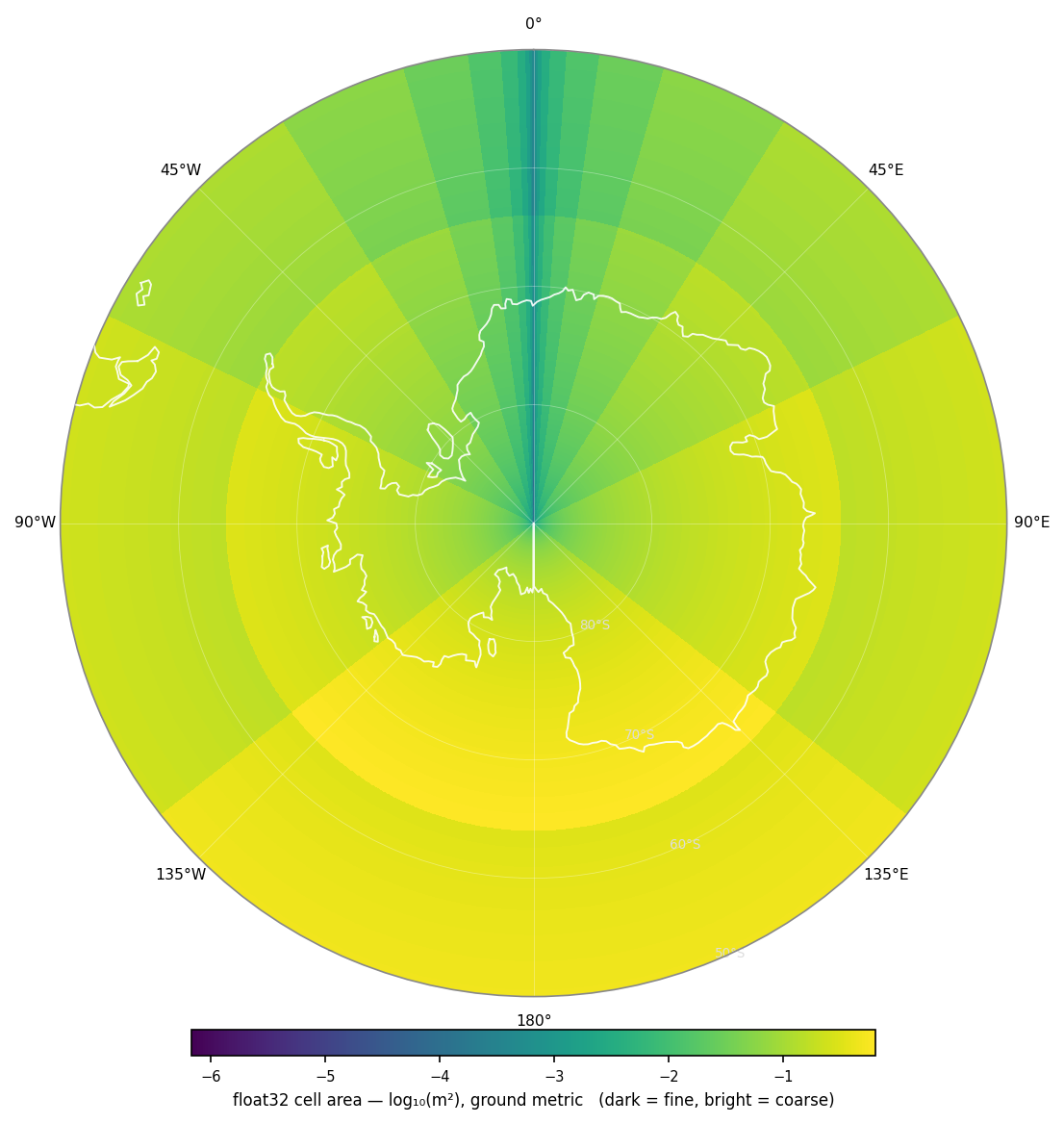
If we zoom way in on the south pole, the lattice of representable lat/lons degenerates into a kind of pie shape:

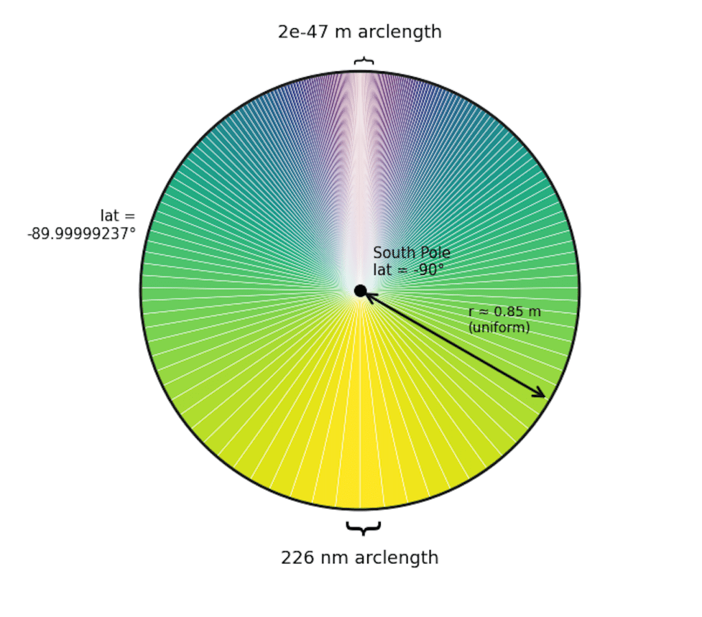
Thinking about this in terms of float32 points, the south pole itself is representable, along with about two billion points around the next representable parallel of $lat = -89.99999237° = -(90 – ULP(90))°$. This parallel can be described physically as the circle of radius ~ 0.85m around the South Pole.

The representable points on this circle are not uniformly distributed. Near the International Date Line (the line extending from the center down to the bottom of the circle), the arc length between representable points corresponds to a physical distance of about 226 nanometers. Near the Prime Meridian (the line extending upwards from the center in the image), the spacing between points corresponds to a physical distance of ~$2*10^{-47}$ meters, or about a trillion times smaller than the Planck Length!

Takeaway

Floating point has many advantages, especially with respect to computational libraries which do things like calculate great circle distances. However, for the sole purpose of representing a set of evenly spaced points on the surface of the Earth, one might be better served by use of a fixed-point type, as this is closer to the spirit of what you actually want; there is nothing particularly special in the physical world about the equator, prime meridian, or poles. Alternatively, coordinate systems like Google’s S2 library are able to cover the surface of the Earth with 2^64 points in a manner which avoids any degeneracies at all; there is some variation in physical precision, but nothing this extreme. Either way, you’re spending the same 64-bit budget; the only difference is where the points land.

1. For the record, all of this is in the context of an idealized earth. The fact is, even if you had an infinitely precise pair of real lat/lon numbers, determining the actual physical point on Earth’s surface this represents is itself kind of meaningless. E.g. the WGS 84 is only well-defined to roughly centimeter precision, and has to be periodically updated to take into account shifts of tectonic plates! ↩︎
2. This image was not generated in a mathematically precise manner, but should be roughly accurate. ↩︎